Background
The NBDCtools R package makes use of the regular
structure of NBDC datasets, especially standardized metadata (data
dictionary and levels table; see, e.g., here)
and the organization of tabulated data as one file per table in the BIDS
rawdata/phenotype/ directory (see here
for information about the structure of the ABCD file-based data, and here
for the HBCD study).
The package assumes that users downloaded the complete tabulated dataset as file-based data and saved the files in a local directory. Using functions from the package, users can then create custom datasets by specifying the study name and any set of variable names and/or table names in its data dictionary.
By making use of the study’s metadata, the functions automatically retrieve the needed columns from different files on disk, and join them to a data frame in memory. This provides a fast, storage- and memory-efficient, and highly reproducible way to work with data from the NBDC Data Hub that can be used as an alternative to creating and downloading different datasets (and creating on-disk representations for each of them) through the Data Exploration & Analysis Portal (DEAP) or the NBDC Data Access Platform.
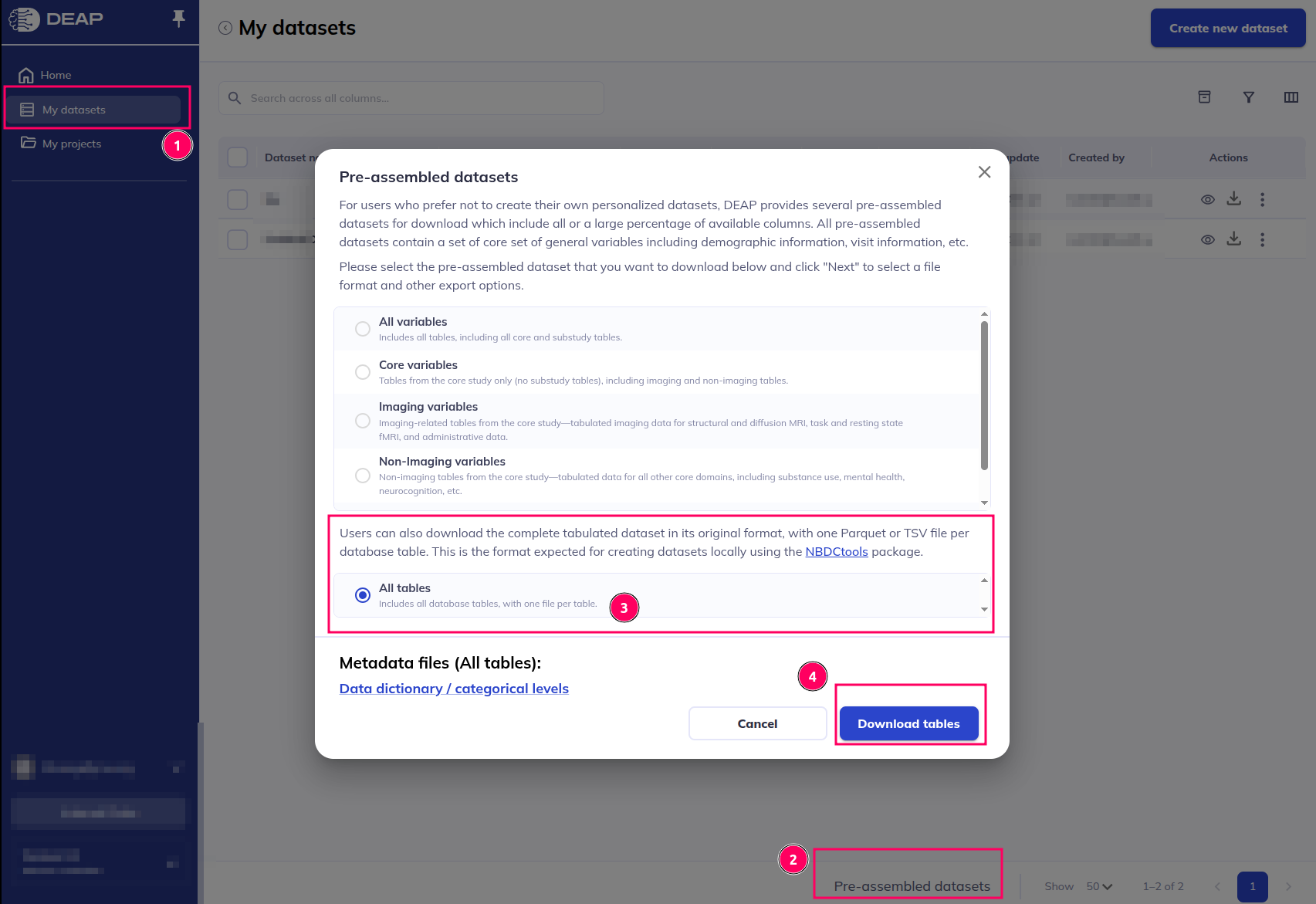
Download data using DEAP
To download data from the NBDC Data Hub in the format that is
required by the NBDCtools package, follow the following
steps:
- Log in to the DEAP
application and select the
My datasetstab. - On the bottom of the page, click on
Pre-assembled datasets. - In the pop-up window, select the
All tablesoption. - Click on the
Download tablesbutton to download the data files. - Unzip the downloaded file to a local directory and remember the path
to this directory, as you will need it to load the data using the
NBDCtoolspackage.
Getting started
To begin using the NBDCtools package effectively, the
most essential and frequently utilized function is
create_dataset(). This omnibus function loads selected
variables from files and creates an analysis-ready data frame in one
step, incorporating various transformation and cleaning options.
In this vignette, we will demonstrate the use of the
create_dataset() function with simulated ABCD data files.
We will illustrate how to join variables, perform various
transformations, and explore some advanced options.
Setup
IMPORTANT: Please ensure that the both the
NBDCtoolsandNBDCtoolsDatapackages are installed. WhenNBDCtoolsis loaded, it will automatically load the required objects fromNBDCtoolsDatapackage, so you don’t need to load it separately.
To load NBDCtools, use the following command:
library(NBDCtools)
#> Welcome to the `NBDCtools` package! For more information, visit: https://software.nbdc-datahub.org/NBDCtools/
#> This package is developed by the ABCD Data Analysis, Informatics & Resource Center (DAIRC) at the J. Craig Venter Institute (JCVI)
Alternatively, you can call functions directly without loading the
package by using ::, e.g.,
NBDCtools::name_of_function(...). You can also access
NBDCtoolsData objects directly using the colon-colon
syntax.
Load and join data
We can use the following command to inspect the simulated data files:
dir_abcd <- system.file("extdata", "phenotype", package = "NBDCtools")
list.files(dir_abcd)
#> [1] "ab_g_dyn.parquet"           "ab_g_stc.parquet"
#> [3] "mr_y_qc__raw__dmri.parquet"
Next, we will use the create_dataset() function to load
data from the files in dir_abcd with selected variables of
interest.
vars <- c(
  "ab_g_dyn__visit_type",
  "ab_g_dyn__cohort_grade",
  "ab_g_dyn__visit__day1_dt",
  "ab_g_stc__gen_pc__01",
  "ab_g_dyn__visit_age",
  "ab_g_dyn__visit_days",
  "ab_g_dyn__visit_dtt",
  "mr_y_qc__raw__dmri__r01__series_t"
)
create_dataset(
  dir_data = dir_abcd,
  study = "abcd",
  vars = vars
)
#> ℹ Loading the data from the "/home/runner/.cache/R/renv/library/NBDCtools-2ca88…
#> ℹ Using metadata "abcd" version "6.0" to join data
#> ✔ Using metadata "abcd" version "6.0" to join data [293ms]
#>
#> ℹ Loading the data from the "/home/runner/.cache/R/renv/library/NBDCtools-2ca88…ℹ Joining 8 variables from 3 tables...
#> ✔ Joining 8 variables from 3 tables... [192ms]
#>
#> ℹ Loading the data from the "/home/runner/.cache/R/renv/library/NBDCtools-2ca88…✔ Loading the data from the "/home/runner/.cache/R/renv/library/NBDCtools-2ca88…
#>
#> ℹ Converting categorical variables to factors.
#> ✔ Converting categorical variables to factors. [122ms]
#>
#> ℹ Adding variable and value labels.
#> ✔ Adding variable and value labels. [229ms]
#>
#> ✔ A dataset with 10 rows and 10 columns has been created. Time used: 0.02
#>   minutes.
#> # A tibble: 10 × 10
#>    participant_id session_id ab_g_dyn__visit_type ab_g_dyn__cohort_grade
#>    <chr>          <fct>      <fct>                <ord>
#>  1 sub-0000000001 ses-02A    1                    NA
#>  2 sub-0000000002 ses-03A    1                    NA
#>  3 sub-0000000003 ses-01A    1                    7
#>  4 sub-0000000004 ses-04A    2                    8
#>  5 sub-0000000005 ses-01A    2                    8
#>  6 sub-0000000006 ses-04A    3                    9
#>  7 sub-0000000007 ses-05A    1                    6
#>  8 sub-0000000008 ses-03A    3                    NA
#>  9 sub-0000000009 ses-00S    3                    8
#> 10 sub-0000000010 ses-04A    3                    8
#> # ℹ 6 more variables: ab_g_dyn__visit__day1_dt <date>,
#> #   ab_g_stc__gen_pc__01 <dbl>, ab_g_dyn__visit_age <dbl>,
#> #   ab_g_dyn__visit_days <int>, ab_g_dyn__visit_dtt <dttm>,
#> #   mr_y_qc__raw__dmri__r01__series_t <chr>
NOTE: The simulated data contains only a few variables and rows. In a real-world scenario, each file will typically have many more rows and tables.
Users can select which variables to join using the following four arguments:
-
vars: Individual variables of interest -
tables: Full tables of interest -
vars_add: Additional individual variables -
tables_add: Additional full tables
Columns of interest specified by the vars and
tables arguments are full-joined, meaning the resulting
data frame retains all rows with at least one non-missing value in the
selected variables/tables. Additional columns specified by the
vars_add and tables_add arguments are
left-joined to the data frame containing the columns of interest,
retaining all rows and adding columns from the additional
variables/tables. The create_dataset() function utilizes
the low-level function join_tabulated() for data joining.
For more information about the join_tabulated() function,
refer to the Join
data vignette. For a diagram detailing the joining strategy for main
and additional variables/tables, see this
page (the NBCDtools package uses the same approach as
the DEAP application).
For example, if we only specify the mr_y_qc__raw__dmri
variable in vars and move others to vars_add,
we will have different number of rows in the data:
create_dataset(
dir_data = dir_abcd,
study = "abcd",
vars = c(
"mr_y_qc__raw__dmri__r01__series_t"
),
vars_add = c(
"ab_g_dyn__visit_type",
"ab_g_dyn__cohort_grade",
"ab_g_dyn__visit__day1_dt",
"ab_g_stc__gen_pc__01",
"ab_g_dyn__visit_age",
"ab_g_dyn__visit_days",
"ab_g_dyn__visit_dtt"
)
)
#> ℹ Loading the data from the "/home/runner/.cache/R/renv/library/NBDCtools-2ca88…
#> ℹ Using metadata "abcd" version "6.0" to join data
#> ✔ Using metadata "abcd" version "6.0" to join data [72ms]
#>
#> ℹ Loading the data from the "/home/runner/.cache/R/renv/library/NBDCtools-2ca88…ℹ Joining 8 variables (1 main; 7 additional) from 3 tables
#> ✔ Joining 15 variables (8 main; 7 additional) from 3 tables [106ms]
#>
#> ℹ Loading the data from the "/home/runner/.cache/R/renv/library/NBDCtools-2ca88…✔ Loading the data from the "/home/runner/.cache/R/renv/library/NBDCtools-2ca88…
#>
#> ℹ Converting categorical variables to factors.
#> ✔ Converting categorical variables to factors. [116ms]
#>
#> ℹ Adding variable and value labels.
#> ✔ Adding variable and value labels. [223ms]
#>
#> ✔ A dataset with 7 rows and 10 columns has been created. Time used: 0.01
#> minutes.
#> # A tibble: 7 × 10
#> participant_id session_id mr_y_qc__raw__dmri__r01__seri…¹ ab_g_dyn__visit_type
#> <chr> <fct> <chr> <fct>
#> 1 sub-0000000002 ses-03A 16:45:46 1
#> 2 sub-0000000003 ses-01A 11:05:35 1
#> 3 sub-0000000004 ses-04A 11:05:35 2
#> 4 sub-0000000005 ses-01A 16:45:46 2
#> 5 sub-0000000008 ses-03A 10:14:34 3
#> 6 sub-0000000009 ses-00S 15:47:35 3
#> 7 sub-0000000010 ses-04A 15:47:35 3
#> # ℹ abbreviated name: ¹mr_y_qc__raw__dmri__r01__series_t
#> # ℹ 6 more variables: ab_g_dyn__cohort_grade <ord>,
#> # ab_g_dyn__visit__day1_dt <date>, ab_g_stc__gen_pc__01 <dbl>,
#> # ab_g_dyn__visit_age <dbl>, ab_g_dyn__visit_days <int>,
#> # ab_g_dyn__visit_dtt <dttm>Process data
After loading and joining the data, the create_dataset()
function performs several transformation steps. Each step is reported
with an i message in the console, allowing users to see
which actions are being taken. For example, the output indicates that
the function has executed the following steps:
#> ℹ Converting categorical variables to factors.
#> ℹ Adding variable and value labels.
These steps utilize lower-level functions that can be used independently. The Transform data vignette describes how to do so.
Default transformations
By default, create_dataset() performs the following two
transformation steps (users can choose to not execute them by setting
the respective arguments to FALSE):
-
categ_to_factor: Converts categorical columns to factors using the lower-level functiontransf_factor(). -
add_labels: Adds variable and value labels using the lower-level functiontransf_label().
Additional transformations
Users can also apply additional transformations to the data by
setting the respective arguments to TRUE. The following
transformations are available:
-
value_to_label: Converts categorical columns’ numeric values to labels using the lower-level functiontransf_value_to_label(). -
value_to_na: Converts categorical missingness/non-response codes toNAusing the lower-level functiontransf_value_to_na(). -
time_to_hms: Converts time variables tohmsclass using the lower-level functiontransf_time_to_hms().
Here is an example of adding these additional transformations to the
create_dataset() function:
create_dataset(
  dir_data = dir_abcd,
  study = "abcd",
  vars = vars,
  value_to_label = TRUE,
  value_to_na = TRUE,
  time_to_hms = TRUE
)
#> ℹ Loading the data from the "/home/runner/.cache/R/renv/library/NBDCtools-2ca88…
#> ℹ Using metadata "abcd" version "6.0" to join data
#> ✔ Using metadata "abcd" version "6.0" to join data [32ms]
#>
#> ℹ Loading the data from the "/home/runner/.cache/R/renv/library/NBDCtools-2ca88…ℹ Joining 8 variables from 3 tables...
#> ✔ Joining 8 variables from 3 tables... [152ms]
#>
#> ℹ Loading the data from the "/home/runner/.cache/R/renv/library/NBDCtools-2ca88…✔ Loading the data from the "/home/runner/.cache/R/renv/library/NBDCtools-2ca88…
#>
#> ℹ Converting categorical variables to factors.
#> ✔ Converting categorical variables to factors. [114ms]
#>
#> ℹ Adding variable and value labels.
#> ✔ Adding variable and value labels. [233ms]
#>
#> ℹ Converting categorical variables' numeric values to labels.
#> ✔ Converting categorical variables' numeric values to labels. [20ms]
#>
#> ℹ Converting categorical missingness/non-response codes to "NA".
#> ✔ Converting categorical missingness/non-response codes to "NA". [93ms]
#>
#> ℹ Converting time variables to <hms> class.
#> ✔ Converting time variables to <hms> class. [86ms]
#>
#> ✔ A dataset with 10 rows and 10 columns has been created. Time used: 0.02
#>   minutes.
#> # A tibble: 10 × 10
#>    participant_id session_id ab_g_dyn__visit_type ab_g_dyn__cohort_grade
#>    <chr>          <fct>      <fct>                <ord>
#>  1 sub-0000000001 ses-02A    On-site              NA
#>  2 sub-0000000002 ses-03A    On-site              NA
#>  3 sub-0000000003 ses-01A    On-site              7th grade
#>  4 sub-0000000004 ses-04A    Remote               8th grade
#>  5 sub-0000000005 ses-01A    Remote               8th grade
#>  6 sub-0000000006 ses-04A    Hybrid               9th grade
#>  7 sub-0000000007 ses-05A    On-site              6th grade
#>  8 sub-0000000008 ses-03A    Hybrid               NA
#>  9 sub-0000000009 ses-00S    Hybrid               8th grade
#> 10 sub-0000000010 ses-04A    Hybrid               8th grade
#> # ℹ 6 more variables: ab_g_dyn__visit__day1_dt <date>,
#> #   ab_g_stc__gen_pc__01 <dbl>, ab_g_dyn__visit_age <dbl>,
#> #   ab_g_dyn__visit_days <int>, ab_g_dyn__visit_dtt <dttm>,
#> #   mr_y_qc__raw__dmri__r01__series_t <time>
Shadow matrices
The create_dataset() function also includes the option
to process shadow matrices. Shadow matrices are tables with the same
dimensions as the original data and provide information about why a
given cell is missing in the original data. Using the
bind_shadow = TRUE argument, users can append the shadow
matrix as additional columns to the end of the data frame.
create_dataset(
  dir_data = dir_abcd,
  study = "abcd",
  vars = vars,
  bind_shadow = TRUE
)
Please note that shadow matrices are processed differently for ABCD and HBCD study datasets:
ABCD: Currently, no raw shadow matrix data is being released. As such,
create_dataset()will create a shadow matrix from the data usingnaniar::as_shadow()ifbind_shadowis set toTRUE.-
HBCD: The shadow matrix is provided as a separate file in the
rawdata/phenotype/directory. Thecreate_dataset()function will read it from the file and append it to the data frame by default ifbind_shadowis set toTRUE. Users can use the additional argumentnaniar_shadow = TRUEif they prefer for the shadow matrix to be created from the data usingnaniar::as_shadow()instead:create_dataset( dir_data = dir_abcd, study = "abcd", vars = vars, bind_shadow = TRUE, naniar_shadow = TRUE )
IMPORTANT: The
naniar::as_shadow()requires thenaniarpackage to be installed, which is not a dependency ofNBDCtools. If you want to use this option, please install thenaniarpackage first usinginstall.packages("naniar").
For more information about shadow matrices, please refer to the Work with shadow matrices vignette.
Advanced options
The create_dataset() function calls several other
low-level functions to process the data. Some of these low-level
functions have additional arguments that can be used to customize the
processing. To use these arguments, users can pass them to the
create_dataset() function using the ...
argument.
For example, if we select value_to_na = TRUE, the
function will call the lower-level transf_value_to_na()
function, which will convert factor levels that represent
missingness/non-response codes to NA. This is useful when
the data contains specific codes that indicate missingness like in the
ABCD study where "222", "333",
"444", etc. are used consistently (see, here
for more details).
One can change the non-response/missingness codes that should be
converted to NA by passing the missing_codes
argument to the create_dataset() function. For example, if
we want to convert the levels 1 and 2 to
NA (this is typically not advisable in a real-world
scenario), we can do so by passing the missing_codes
argument to the create_dataset() function as follows:
create_dataset(
  dir_data = dir_abcd,
  study = "abcd",
  vars = vars,
  value_to_na = TRUE,
  missing_codes = c("1", "2")
)
#> ℹ Loading the data from the "/home/runner/.cache/R/renv/library/NBDCtools-2ca88…
#> ℹ Using metadata "abcd" version "6.0" to join data
#> ✔ Using metadata "abcd" version "6.0" to join data [34ms]
#>
#> ℹ Loading the data from the "/home/runner/.cache/R/renv/library/NBDCtools-2ca88…ℹ Joining 8 variables from 3 tables...
#> ✔ Joining 8 variables from 3 tables... [155ms]
#>
#> ℹ Loading the data from the "/home/runner/.cache/R/renv/library/NBDCtools-2ca88…✔ Loading the data from the "/home/runner/.cache/R/renv/library/NBDCtools-2ca88…
#>
#> ℹ Converting categorical variables to factors.
#> ✔ Converting categorical variables to factors. [117ms]
#>
#> ℹ Adding variable and value labels.
#> ✔ Adding variable and value labels. [223ms]
#>
#> ℹ Converting categorical missingness/non-response codes to "NA".
#> ℹ Argument `missing_codes` is passed to `transf_value_to_na()`.
#> ✔ Argument `missing_codes` is passed to `transf_value_to_na()`. [11ms]
#>
#> ℹ Converting categorical missingness/non-response codes to "NA".✔ Converting categorical missingness/non-response codes to "NA". [111ms]
#>
#> ✔ A dataset with 10 rows and 10 columns has been created. Time used: 0.01
#>   minutes.
#> # A tibble: 10 × 10
#>    participant_id session_id ab_g_dyn__visit_type ab_g_dyn__cohort_grade
#>    <chr>          <fct>      <fct>                <ord>
#>  1 sub-0000000001 ses-02A    NA                   NA
#>  2 sub-0000000002 ses-03A    NA                   NA
#>  3 sub-0000000003 ses-01A    NA                   7
#>  4 sub-0000000004 ses-04A    NA                   8
#>  5 sub-0000000005 ses-01A    NA                   8
#>  6 sub-0000000006 ses-04A    3                    9
#>  7 sub-0000000007 ses-05A    NA                   6
#>  8 sub-0000000008 ses-03A    3                    NA
#>  9 sub-0000000009 ses-00S    3                    8
#> 10 sub-0000000010 ses-04A    3                    8
#> # ℹ 6 more variables: ab_g_dyn__visit__day1_dt <date>,
#> #   ab_g_stc__gen_pc__01 <dbl>, ab_g_dyn__visit_age <dbl>,
#> #   ab_g_dyn__visit_days <int>, ab_g_dyn__visit_dtt <dttm>,
#> #   mr_y_qc__raw__dmri__r01__series_t <chr>
First create_dataset() prints out the message that
indicating which additional arguments are passed to the low-level
functions:
#> ℹ Argument `missing_codes` is passed to `transf_value_to_na()`.In the results, we can see that in column
ab_g_dyn__visit_type, the levels 1 and
2 are converted to NA, while the other values
are kept as is.
If the user defines wrong or not existing arguments, they will be
ignored. For example, if we pass an additional argument
my_arg to create_dataset() function, it will
be ignored and the returned data will be the same as if we did not pass
this argument at all:
create_dataset(
  dir_data = dir_abcd,
  study = "abcd",
  vars = vars,
  value_to_na = TRUE,
  my_arg = "some_value" # this argument will be ignored
)
#> ℹ Loading the data from the "/home/runner/.cache/R/renv/library/NBDCtools-2ca88…
#> ℹ Using metadata "abcd" version "6.0" to join data
#> ✔ Using metadata "abcd" version "6.0" to join data [32ms]
#>
#> ℹ Loading the data from the "/home/runner/.cache/R/renv/library/NBDCtools-2ca88…ℹ Joining 8 variables from 3 tables...
#> ✔ Joining 8 variables from 3 tables... [147ms]
#>
#> ℹ Loading the data from the "/home/runner/.cache/R/renv/library/NBDCtools-2ca88…✔ Loading the data from the "/home/runner/.cache/R/renv/library/NBDCtools-2ca88…
#>
#> ℹ Converting categorical variables to factors.
#> ✔ Converting categorical variables to factors. [111ms]
#>
#> ℹ Adding variable and value labels.
#> ✔ Adding variable and value labels. [223ms]
#>
#> ℹ Converting categorical missingness/non-response codes to "NA".
#> ✔ Converting categorical missingness/non-response codes to "NA". [91ms]
#>
#> ✔ A dataset with 10 rows and 10 columns has been created. Time used: 0.01
#>   minutes.
#> # A tibble: 10 × 10
#>    participant_id session_id ab_g_dyn__visit_type ab_g_dyn__cohort_grade
#>    <chr>          <fct>      <fct>                <ord>
#>  1 sub-0000000001 ses-02A    1                    NA
#>  2 sub-0000000002 ses-03A    1                    NA
#>  3 sub-0000000003 ses-01A    1                    7
#>  4 sub-0000000004 ses-04A    2                    8
#>  5 sub-0000000005 ses-01A    2                    8
#>  6 sub-0000000006 ses-04A    3                    9
#>  7 sub-0000000007 ses-05A    1                    6
#>  8 sub-0000000008 ses-03A    3                    NA
#>  9 sub-0000000009 ses-00S    3                    8
#> 10 sub-0000000010 ses-04A    3                    8
#> # ℹ 6 more variables: ab_g_dyn__visit__day1_dt <date>,
#> #   ab_g_stc__gen_pc__01 <dbl>, ab_g_dyn__visit_age <dbl>,
#> #   ab_g_dyn__visit_days <int>, ab_g_dyn__visit_dtt <dttm>,
#> #   mr_y_qc__raw__dmri__r01__series_t <chr>
Please refer to the lower-level functions documentation for more information about the available arguments and their usage on the Reference page.